Loading and visualizing a mesh

The shortest possible pyFM session: read a triangle mesh from disk, inspect its properties.

Every 3D plot below is interactive.

Locating data

The example meshes are stored in examples/data and are not part of the package.

from pathlib import Path

from pyFM.mesh import TriMesh
from pyFM.viz import plot_mesh


def example_data(name):
    """Return the path to a mesh in the ``examples/data`` folder."""
    for folder in [Path.cwd(), *Path.cwd().parents]:
        candidate = folder / "examples" / "data" / name
        if candidate.exists():
            return candidate
    raise FileNotFoundError(
        f"{name!r} not found. These examples read data from the pyFM repository; "
        "clone it and run them there."
    )

Reading a mesh

load() reads a .off, .obj or .ply file. area_normalize rescales the mesh to unit area and center moves its center of mass to the origin. This is usually desirable. A shortcut with the same effect is the normalize argument.

mesh = TriMesh.load(example_data("cat.obj"), area_normalize=True, center=True)

print(f"{mesh.n_vertices} vertices, {mesh.n_faces} faces")
print(f"total area: {mesh.area:.6f}")

7207 vertices, 14410 faces
total area: 1.000000

Vertices and faces are plain numpy arrays, available as vertices and faces. Other geometric quantities such as normals, face areas, edges, the Laplacian, … are computed the first time you ask for them, and stored afterwards.

print("vertices:", mesh.vertices.shape, mesh.vertices.dtype)
print("faces   :", mesh.faces.shape, mesh.faces.dtype)
print("face areas:", mesh.face_areas.shape)

vertices: (7207, 3) float64
faces   : (14410, 3) int64
face areas: (14410,)

Visualizing

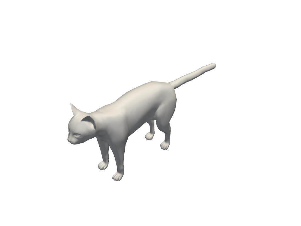
pyFM.viz.plot_mesh renders a mesh. It is part of the optional viz extra (pip install 'pyfmaps[viz]'), which is built on PyVista.

plot_mesh(mesh)

Static Scene

Interactive Scene

Coloring by a scalar field

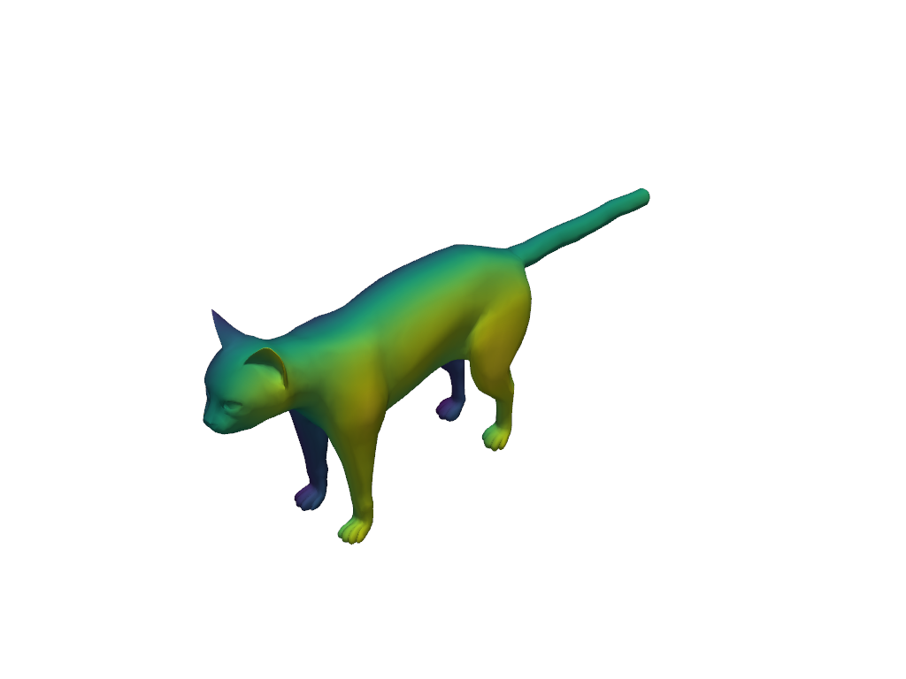
Any per-vertex array can be passed as scalars, and cmap names the matplotlib colormap it is read through. Here we simply use the height of each vertex. Next examples use eigenfunctions of the Laplacian, descriptors or geodesic distances. Per-face arrays work too.

height = mesh.vertices[:, 1]

plot_mesh(mesh, scalars=height, cmap="viridis")

Static Scene

Interactive Scene

Coloring by position

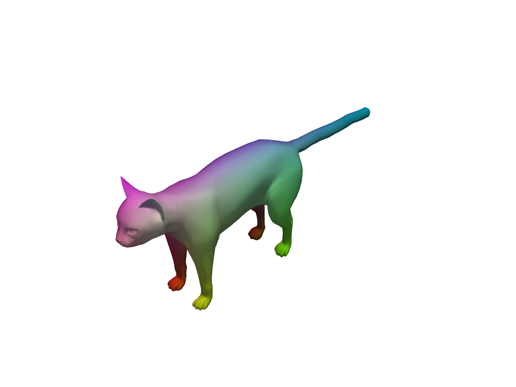
Mapping the (x, y, z) coordinates onto (r, g, b) gives each vertex a color that varies smoothly across the surface. This is a standard way to visualize correspondence. vertices_to_rgb() does this with a better transformation than the plain min/max rescaling below, and is what the later examples use.

lo = mesh.vertices.min(axis=0, keepdims=True)
hi = mesh.vertices.max(axis=0, keepdims=True)
rgb = (mesh.vertices - lo) / (hi - lo)

plot_mesh(mesh, scalars=rgb)

Static Scene

Interactive Scene

Note

rgb here is an (n, 3) float array in [0, 1], which is rendered directly as colors. A one-dimensional (n,) array is interpreted as a scalar field and mapped to colors using the cmap colormap.

print("rgb array:", rgb.shape, f"range [{rgb.min():.2f}, {rgb.max():.2f}]")

rgb array: (7207, 3) range [0.00, 1.00]