Encoding Dense Correspondences in a Functional Map

A functional map is a compact (approximate) representation of correspondences as a small sized matrix. It is simply the pull-back operator of a pointwise map, expressed in the spectral basis of the two shapes.

Representing the correspondence via its pullback is easy and lossless, as it captures all the information of the original pointwise map. The compactness of functional maps comes from reducing this operator to a reduced space, which loses some information.

Setup

The example meshes are stored in examples/data and are not part of the package.

from pathlib import Path

import matplotlib.pyplot as plt
import numpy as np
import pyvista as pv
from scipy import sparse

from pyFM.mesh import TriMesh
from pyFM.spectral import knn_query, mesh_FM_to_p2p, mesh_p2p_to_FM
from pyFM.viz import plot_mesh, vertices_to_rgb


def example_data(name):
    """Return the path to a mesh in the ``examples/data`` folder."""
    for folder in [Path.cwd(), *Path.cwd().parents]:
        candidate = folder / "examples" / "data" / name
        if candidate.exists():
            return candidate
    raise FileNotFoundError(
        f"{name!r} not found. These examples read data from the pyFM repository; "
        "clone it and run them there."
    )


np.random.seed(0)


mesh1 = TriMesh.load(example_data("tr_reg_000.off"), normalize=True).process(k=100)
mesh2 = TriMesh.load(example_data("tr_reg_047.off"), normalize=True).process(k=100)

print(mesh1, mesh2, sep="\n")

<TriMesh 'tr_reg_000': 6890 vertices, 13776 faces>
<TriMesh 'tr_reg_047': 6890 vertices, 13776 faces>

Conventions and representations

Given a map \(\varphi: \mathcal{X}_2 \to \mathcal{X}_1\), the functional map is a representation of the pull-back operator:

\[ \varphi^*: L^2(\mathcal{X}_1) \to L^2(\mathcal{X}_2) \]

Notably, the functional maps and the pointwise maps are in “opposite” directions. Because pyFM focuses on functional maps, we adopt the arbitrary convention that the functional map goes from shape 1 to shape 2. Pointwise maps will then go from shape 2 to shape 1.

In the code this translates to the following shapes:

• FM_12 is the functional map from shape 1 to shape 2, of shape (k2, k1).

• p2p_21 is the pointwise map from shape 2 to shape 1, of shape (n2,): p2p_21[i] is the vertex of shape 1 matching vertex i of shape 2.

To illustrate different representations, we start with the unusual setting where the ground-truth pointwise map is available.

gt_p2p_21 = np.arange(mesh2.n_vertices)

Two helpers used on this page: one to score a map, one to draw it.

Scoring a map means measuring, for each vertex, the geodesic distance on shape 1 between where the map sends it and where it should go. pyFM.eval.accuracy() does this from a full (n1, n1) geodesic matrix, but here we only evaluate on 300 points for speed.

def error_function(mesh1, mesh2, gt_p2p_21, n_samples=300):
    """Return a function scoring a map from shape 2 to shape 1, in percent of sqrt_area."""
    sub = mesh2.farthest_point_sampling(n_samples)
    distances = mesh1.geodesic_from(gt_p2p_21[sub])  # (n1, n_samples)
    columns = np.arange(n_samples)

    def error(p2p_21):
        return 1e2 * distances[p2p_21[sub], columns].mean() / mesh1.sqrt_area

    return error


def show_map(mesh1, mesh2, p2p_21, title=""):
    """Color shape 1 by position, and shape 2 by the colors pulled through the map."""
    colors1 = vertices_to_rgb(mesh1.vertices)
    pl = pv.Plotter(shape=(1, 2))
    pl.subplot(0, 0)
    plot_mesh(mesh1, scalars=colors1, pl=pl)
    pl.add_title("source", font_size=9)
    pl.subplot(0, 1)
    plot_mesh(mesh2, scalars=colors1[p2p_21], pl=pl)
    pl.add_title(title, font_size=9)
    pl.link_views()
    pl.show(cpos="xy")


error = error_function(mesh1, mesh2, gt_p2p_21)

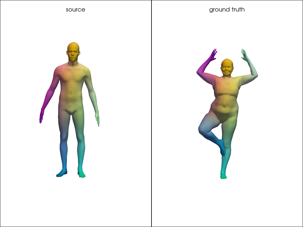
Matching colors mean matching points. Under the ground-truth map the two shapes agree everywhere, which is what a perfect correspondence looks like.

show_map(mesh1, mesh2, gt_p2p_21, "ground truth")

Static Scene

Interactive Scene

What is a functional map

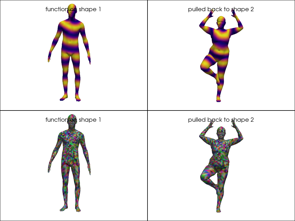
A functional map is simply the pull-back operator of a pointwise map \(\varphi\). What this means is that given a function \(f\) on shape 1, the functional map is a linear map that produces a function \(f \circ \varphi\) on shape 2. What does this mean precisely ? Let’s say we have a function \(f=(f_1, \dots, f_{n_1})\) on shape 1, where \(f_i\) is the value of the function at vertex \(i\) of shape 1. Then the pull-back of \(f\) through the map \(\varphi\) is the function \(\varphi^* f = f \circ \varphi = (f_{\varphi(1)}, \dots, f_{\varphi(n_2)})\) on shape 2. In matrix form we write \(\varphi^* f = \Pi_{21} f\), where \(\Pi_{21}\) is the simple \((n_2, n_1)\) matrix with \(\Pi_{21}[i, j] = 1\) if \(\varphi(i) = j\) and \(0\) otherwise.

This is the standard permutation matrix associated to the pointwise map, with a single value per line. On the example below, we take 2 signals on shape 1, and pull them back through the ground-truth map to shape 2:

• One is a geodesic distance from a vertex of shape 1,

• One is a pure random RGB signal on shape 1.

The result is exactly the same signals, but on shape 2.

P21_gt = sparse.csr_matrix(
    (np.ones(mesh2.n_vertices), (np.arange(mesh2.n_vertices), gt_p2p_21)),
    shape=(mesh2.n_vertices, mesh1.n_vertices),
)

f1 = np.cos(2 * np.pi * mesh1.geodesic_from(300) / 0.2)
f2 = np.random.random((mesh1.n_vertices, 3))

pl = pv.Plotter(shape=(2, 2))
pl.subplot(0, 0)
plot_mesh(mesh1, scalars=f1, cmap="plasma", pl=pl)
pl.add_title("function on shape 1", font_size=9)
pl.subplot(0, 1)
plot_mesh(mesh2, scalars=P21_gt @ f1, cmap="plasma", pl=pl)
pl.add_title("pulled back to shape 2", font_size=9)
pl.subplot(1, 0)
plot_mesh(mesh1, scalars=f2, pl=pl)
pl.add_title("function on shape 1", font_size=9)
pl.subplot(1, 1)
plot_mesh(mesh2, scalars=P21_gt @ f2, pl=pl)
pl.add_title("pulled back to shape 2", font_size=9)
pl.link_views()
pl.show(cpos="xy")

Static Scene

Interactive Scene

The map as a matrix

The functional map shown above is a large sparse matrix of shape (n2, n1), which is the size of the two shapes. So the procedure didn’t compress any information, the pointwise map can be exactly recovered by looking at the positions of the non-zero entries in the matrix.

The thing is that P21_gt is the functional map, expressed in the canonical basis of functions on each shape, that is the basis of delta functions at each vertex \((1,0,\dots,0)^T, (0,1,0,\dots,0)^T, \dots, (0,\dots,0,1)^T\).

By changing the basis of functions on each shape, we can express the same operator as a different (n,n) matrix, which is not a permutation anymore. What we will see is that with a good choice of basis, truncating the matrix to a small size still captures the essence of the map, and can be used to transfer smooth functions between shapes. While the truncated functional map will not be able to transfer all functions, and in particular the random values shown above, it will still be able to transfer smooth functions effectively, which is enough information to recover most of the pointwise map.

Given a basis of functions of size k_i on shape i, where each basis function is a column of the matrix \(\Phi_i\) of size \(n_i \times k_i\), the (truncated) functional map associated to a pointwise map is simply the least-squares solution of \(\Phi_2 C_{12} = \Pi_{21}\Phi_1\), where \(\Pi_{21}\) is the permutation matrix of the pointwise map.

In practice, we select the first \(K\) eigenfunctions of the Laplacian as a basis. Since these eigenfunctions are orthonormal w.r.t the area matrix on each shape, \(\Phi_2^\top A_2 \Phi_2 = I\), the solution has a simple closed form expression

\[C_{12} = \Phi_2^\top A_2 \Pi_{21} \Phi_1\]

where \(A_2\) is the area matrix of shape 2.

In the following, a functional map is always assumed to be expressed in the truncated Laplacian basis of the two shapes, unless specified otherwise.

In the code, mesh_p2p_to_FM() expresses a pointwise map in the two spectral bases. dims=k gives a (k, k) matrix; dims=(k1, k2) gives a rectangular (k2, k1) one.

FM_12 = mesh_p2p_to_FM(gt_p2p_21, mesh1, mesh2, dims=50)

print(f"functional map: {FM_12.shape}, from {mesh1.n_vertices} x {mesh2.n_vertices} indices")

functional map: (50, 50), from 6890 x 6890 indices

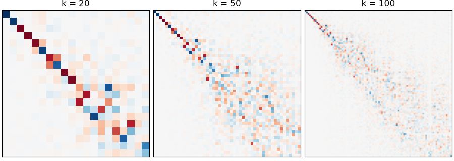
The matrix concentrates near the diagonal, which is a signature of a near-isometric pair: low-frequency eigenfunctions of one shape are combinations of the low-frequency eigenfunctions of the other. A correspondence between unrelated shapes has no such structure.

fig, axes = plt.subplots(1, 3, figsize=(9, 3.2), constrained_layout=True)
for ax, k in zip(axes, [20, 50, 100]):
    C = mesh_p2p_to_FM(gt_p2p_21, mesh1, mesh2, dims=k)
    bound = np.abs(C).max()
    ax.imshow(C, cmap="RdBu_r", vmin=-bound, vmax=bound)
    ax.set_title(f"k = {k}")
    ax.set_xticks([])
    ax.set_yticks([])
plt.show()

And back again

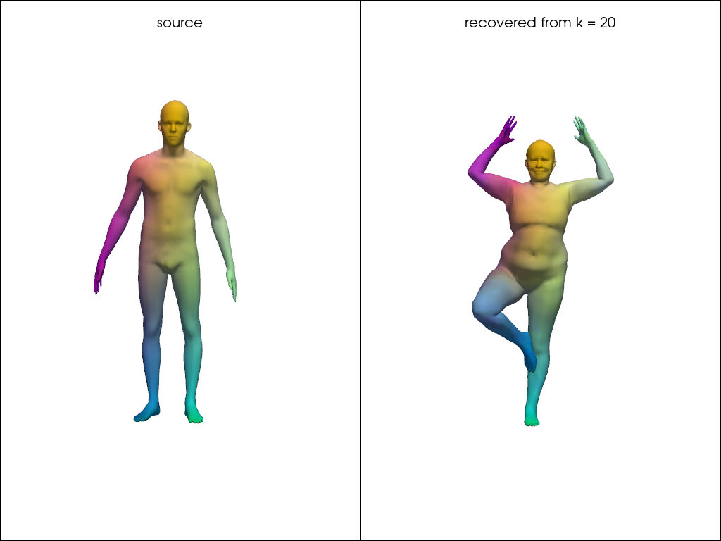
mesh_FM_to_p2p() recovers a vertex map, by nearest neighbours in the spectral embedding. The round trip is lossy as the matrix only holds what the first k eigenfunctions can express. Errors below are mean geodesic errors, in percent of \(\sqrt{\text{area}}\).

for k in [5, 20, 50, 100]:
    C = mesh_p2p_to_FM(gt_p2p_21, mesh1, mesh2, dims=k)
    print(f"k = {k:3d}: error after the round trip = {error(mesh_FM_to_p2p(C, mesh1, mesh2)):.2f}")

k =   5: error after the round trip = 8.98
k =  20: error after the round trip = 3.37
k =  50: error after the round trip = 1.46
k = 100: error after the round trip = 0.57

At k = 20 the error is already small, so the whole correspondence is essentially encoded in a 20x20 matrix, whatever the number of vertices. use_adj=True switches mesh_FM_to_p2p() to the adjoint formulation, which is the mathematically correct one and usually a little better behaved.

C_20 = mesh_p2p_to_FM(gt_p2p_21, mesh1, mesh2, dims=20)
show_map(mesh1, mesh2, mesh_FM_to_p2p(C_20, mesh1, mesh2), "recovered from k = 20")

Static Scene

Interactive Scene

Transferring a function

The point of the small matrix is that it acts on functions rather than on points: project on shape 1, multiply, unproject on shape 2. No pointwise map is involved.

f1 = np.cos(2 * np.pi * mesh1.geodesic_from(400) / 0.6)
f2 = mesh2.unproject(FM_12 @ mesh1.project(f1, k=FM_12.shape[1]))

print(f"{f1.shape} -> {mesh1.project(f1, k=50).shape} coefficients -> {f2.shape}")

pl = pv.Plotter(shape=(1, 2))
pl.subplot(0, 0)
plot_mesh(mesh1, scalars=f1, cmap="plasma", pl=pl)
pl.add_title("function on shape 1", font_size=9)
pl.subplot(0, 1)
plot_mesh(mesh2, scalars=f2, cmap="plasma", pl=pl)
pl.add_title("transferred to shape 2", font_size=9)
pl.link_views()
pl.show(cpos="xy")

Static Scene

Interactive Scene

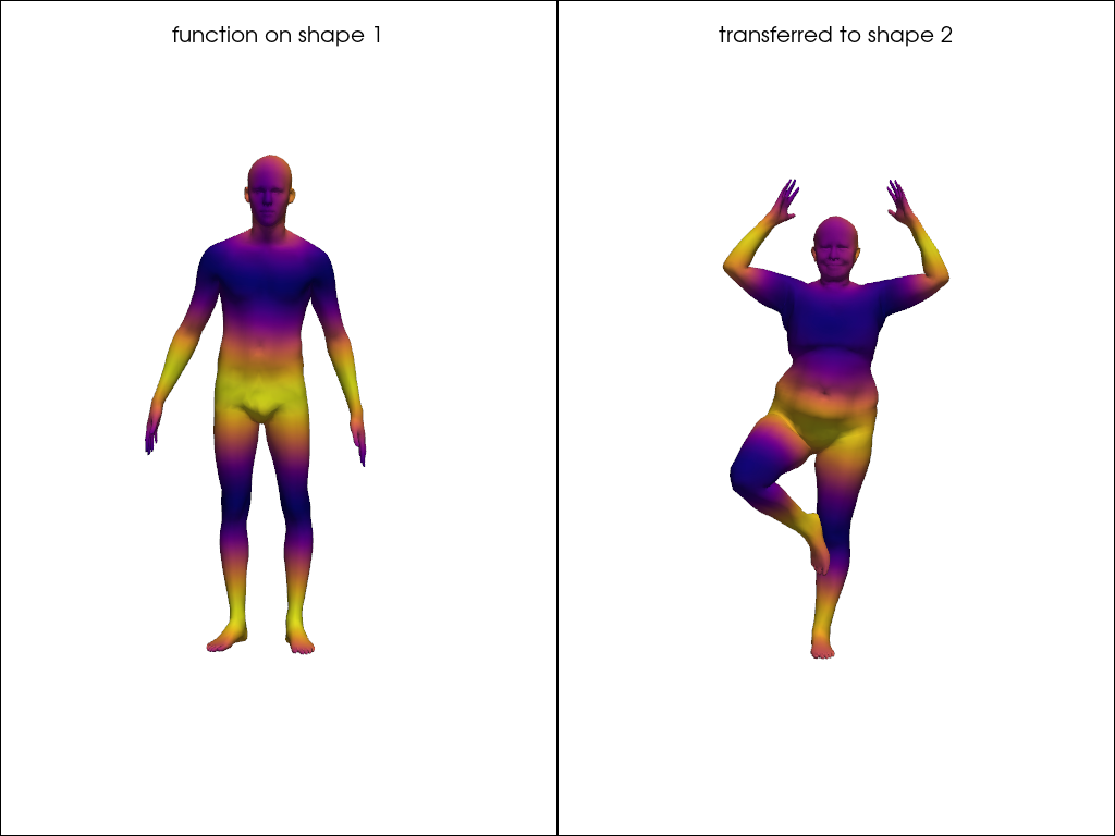
(6890,) -> (50,) coefficients -> (6890,)

transfer() wraps these three steps.

Initialization by nearest neighbours

Everything above used the ground-truth map as input, which is exactly what we do not have in practice. So where does a first \(\Pi_{21}\) come from ?

The cheapest answer is to match each vertex of shape 2 to the closest vertex of shape 1 in \(\mathbb{R}^3\). This compares positions, so it only means something if the two shapes are already aligned. Here, tr_reg_040 is another subject in the same pose as tr_reg_000, so this is the favourable case.

mesh_aligned = TriMesh.load(example_data("tr_reg_040.off"), normalize=True)
error_aligned = error_function(mesh1, mesh_aligned, np.arange(mesh_aligned.n_vertices))

p2p_nn_aligned = knn_query(mesh1.vertices, mesh_aligned.vertices, k=1)

print(f"nearest neighbours, same pose     : {error_aligned(p2p_nn_aligned):.2f}")

show_map(mesh1, mesh_aligned, p2p_nn_aligned, "nearest neighbours, same pose")

Static Scene

Interactive Scene

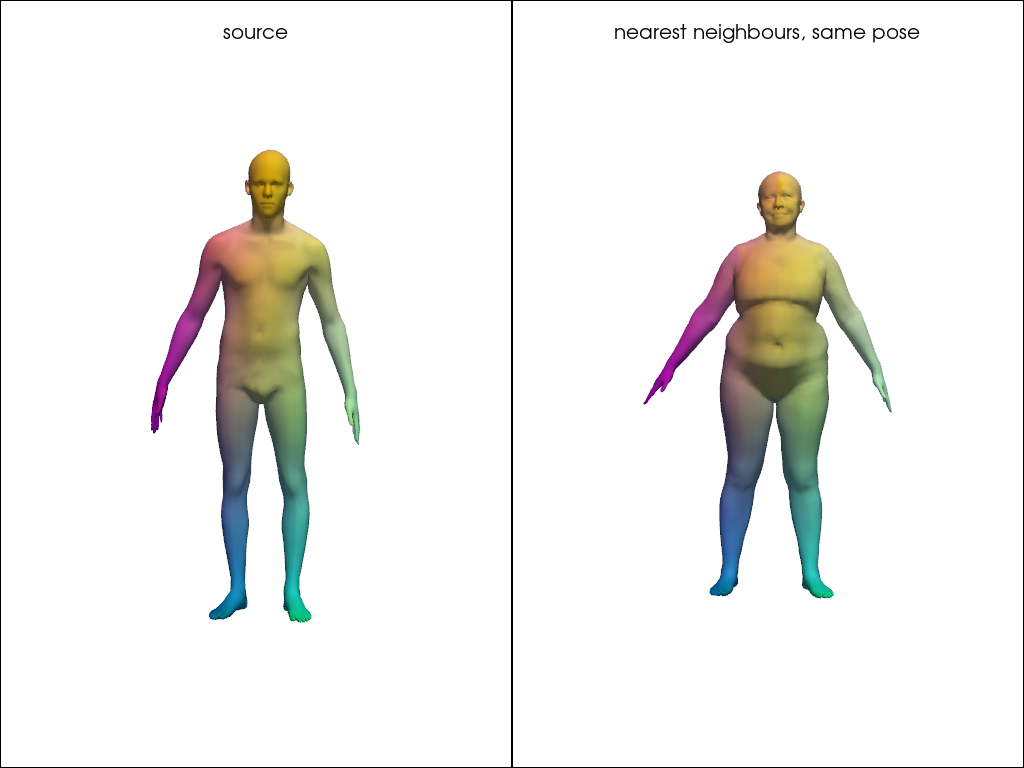
nearest neighbours, same pose     : 3.43

The map is noisy up close but globally right, which is all we need from an initialization.

tr_reg_047 is the same subject as tr_reg_040, in a different pose. The exact same call now returns something unrelated to the true map: an arm folded across the body picks up the colors of the torso, since that is what is nearby.

p2p_nn = knn_query(mesh1.vertices, mesh2.vertices, k=1)

print(f"nearest neighbours, different pose: {error(p2p_nn):.2f}")

show_map(mesh1, mesh2, p2p_nn, "nearest neighbours, different pose")

Static Scene

Interactive Scene

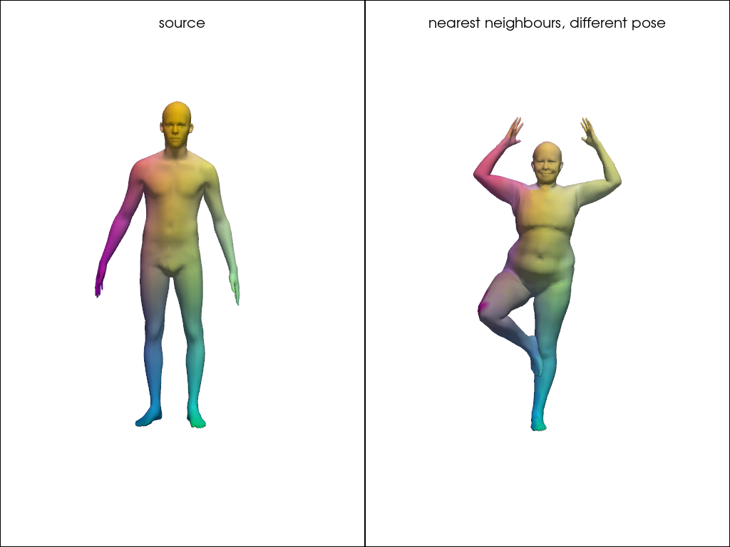
nearest neighbours, different pose: 22.83

Initialization from landmarks

When the shapes are not aligned, a handful of matched points is enough to get a small map.

The idea is the same least-squares problem as above, but written only on the rows we know. With \(p\) landmarks on each shape, we solve \(\Phi_2[\text{lmks}_2] C_{12} = \Phi_1[\text{lmks}_1]\), which is \(p\) equations for \(k_2\) unknowns per column of \(C_{12}\). This only determines \(C_{12}\) if \(k_2 \leq p\), so a few landmarks buy a small map, and only a small one.

In the code this is subsample=(lmks1, lmks2), which tells mesh_p2p_to_FM() that the correspondence is only known on those vertices. The area matrix is dropped and the system is solved by least squares.

Note we use here the same indices on both shapes, which is only valid because this pair shares its triangulation. In general landmarks come as pairs of indices, as in examples/data/landmarks.txt.

for n_landmarks, k in [(20, 10), (20, 20), (50, 20), (50, 30)]:
    lmks = mesh1.farthest_point_sampling(n_landmarks)
    C_lmk = mesh_p2p_to_FM(
        np.arange(n_landmarks), mesh1, mesh2, dims=(k, k), subsample=(lmks, lmks)
    )
    p2p_lmk = mesh_FM_to_p2p(C_lmk, mesh1, mesh2)
    print(f"{n_landmarks:3d} landmarks, k = {k:2d}: {error(p2p_lmk):.2f}")

20 landmarks, k = 10: 6.67
20 landmarks, k = 20: 14.59
50 landmarks, k = 20: 3.56
50 landmarks, k = 30: 3.76

50 landmarks and a 20x20 matrix already do much better than nearest neighbours on this pair, on shapes with no alignment at all. Note this is about what the ground-truth map gave above. This means that 50 well spread points are enough to recover a 20x20 map almost as well as knowing correspondences for every single vertex.

Taking \(k\) all the way up to \(p\) actually makes things worse, not better. The system becomes square and fits the landmarks exactly, which is somehow noisy as we don’t expect the truncated functional map to exactly fit landmarks.

Note

With very few landmarks, this is probably not the way to go. Prefer fit(), which treats landmarks as soft constraints and leaves \(k\) free, then ZoomOut. See Computing a map without a correspondence.

lmks = mesh1.farthest_point_sampling(50)
C_lmk = mesh_p2p_to_FM(np.arange(50), mesh1, mesh2, dims=(20, 20), subsample=(lmks, lmks))
p2p_lmk = mesh_FM_to_p2p(C_lmk, mesh1, mesh2)

colors1 = vertices_to_rgb(mesh1.vertices)

pl = pv.Plotter(shape=(1, 2))
pl.subplot(0, 0)
plot_mesh(mesh1, scalars=colors1, points=lmks, points_color="black", point_size=10, pl=pl)
pl.add_title("source, 50 landmarks", font_size=9)
pl.subplot(0, 1)
plot_mesh(mesh2, scalars=colors1[p2p_lmk], points=lmks, points_color="black", point_size=10, pl=pl)
pl.add_title("from landmarks, k = 20", font_size=9)
pl.link_views()
pl.show(cpos="xy")

Static Scene

Interactive Scene

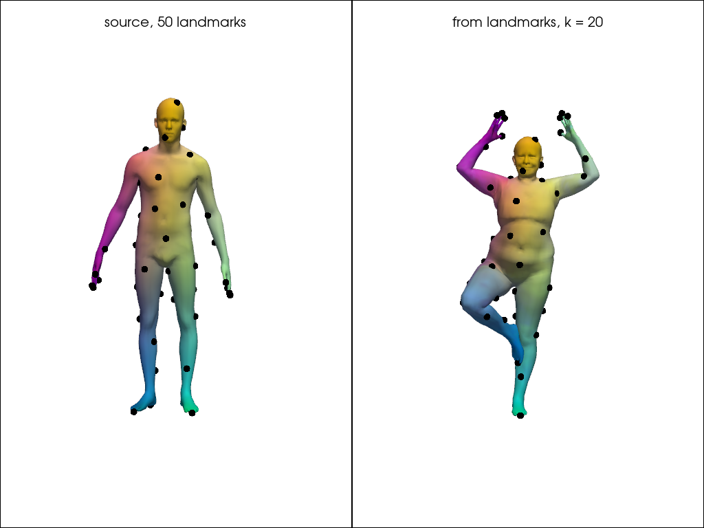
Both of these are initializations, not answers. Computing a map without a correspondence computes a map when neither is available, and refines any of them into something usable.