Geometry of a triangle mesh

Everything a TriMesh knows is derived from two arrays, vertices and faces: edges, areas, normals, geodesic distances. None of it is computed when the mesh is loaded but instead built the first time you ask for it, and stored afterwards.

This page walks through those quantities and plots them with pyFM.viz. Drag to rotate the 3D views, scroll to zoom.

Locating data

The example meshes are stored in examples/data and are not part of the package.

from pathlib import Path

import numpy as np
import pyvista as pv

from pyFM.mesh import TriMesh
from pyFM.viz import plot_arrows, plot_mesh


def example_data(name):
    """Return the path to a mesh in the ``examples/data`` folder."""
    for folder in [Path.cwd(), *Path.cwd().parents]:
        candidate = folder / "examples" / "data" / name
        if candidate.exists():
            return candidate
    raise FileNotFoundError(
        f"{name!r} not found. These examples read data from the pyFM repository; "
        "clone it and run them there."
    )


np.random.seed(0)

Loading a mesh

area_normalize rescales the mesh to unit area and center moves its center of mass to the origin. Scaling is particularly useful for numerical stability of spectral quantities. normalize is a convenient shortcut that applies both area_normalize and center.

mesh = TriMesh.load(example_data("cat.obj"), area_normalize=True, center=True)

print(mesh)
print(f"name: {mesh.name}, loaded from: {Path(mesh.path).name}")
print(f"area: {mesh.area:.6f}, sqrt_area: {mesh.sqrt_area:.6f}")

<TriMesh 'cat': 7207 vertices, 14410 faces>
name: cat, loaded from: cat.obj
area: 1.000000, sqrt_area: 1.000000

Rigid transformations

rotate(), translate(), scale(), center() and area_normalize() modify the mesh in place and return it, so they can be chained. Work on a copy() when you want to keep the original around.

These methods also carry the already-computed quantities along instead of throwing them away. For instance rotating rotates the cached normals, and scale(alpha) rescales the mass matrix, face areas, divides the eigenvalues by alpha**2 and the eigenvectors by alpha. Note that area_normalize preserves the center of mass, so it never moves the shape.

theta = np.pi / 4
rotation = np.array(
    [
        [np.cos(theta), -np.sin(theta), 0],
        [np.sin(theta), np.cos(theta), 0],
        [0, 0, 1],
    ]
)

moved = mesh.copy().scale(0.6).rotate(rotation).translate(np.array([0.3, 0.0, 0.0]))

print(f"original area: {mesh.area:.6f}")
print(f"scaled area  : {moved.area:.6f}  (0.6^2 = {0.6**2:.2f})")

pl = pv.Plotter()
plot_mesh(mesh, color="#91c0d8", pl=pl)
plot_mesh(moved, color="#d27575", pl=pl)
pl.show()

Static Scene

Interactive Scene

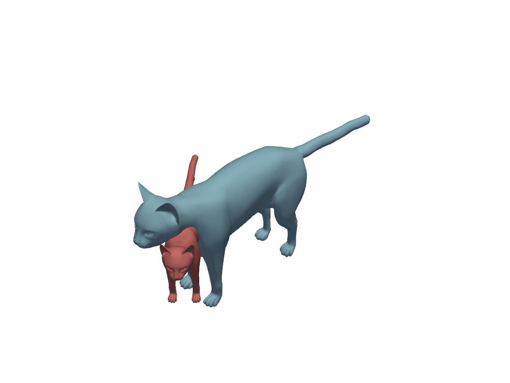
original area: 1.000000
scaled area  : 0.360000  (0.6^2 = 0.36)

Edges and faces

edges lists each undirected edge and edge_lengths gives their lengths. We can confirm the Euler characteristic of a sphere-like shape is 2.

print(f"vertices: {mesh.n_vertices}, edges: {len(mesh.edges)}, faces: {mesh.n_faces}")
print(f"Euler characteristic: {mesh.n_vertices - len(mesh.edges) + mesh.n_faces}")
print(f"mean edge length: {mesh.edge_lengths.mean():.4f}")

vertices: 7207, edges: 21615, faces: 14410
Euler characteristic: 2
mean edge length: 0.0123

Areas

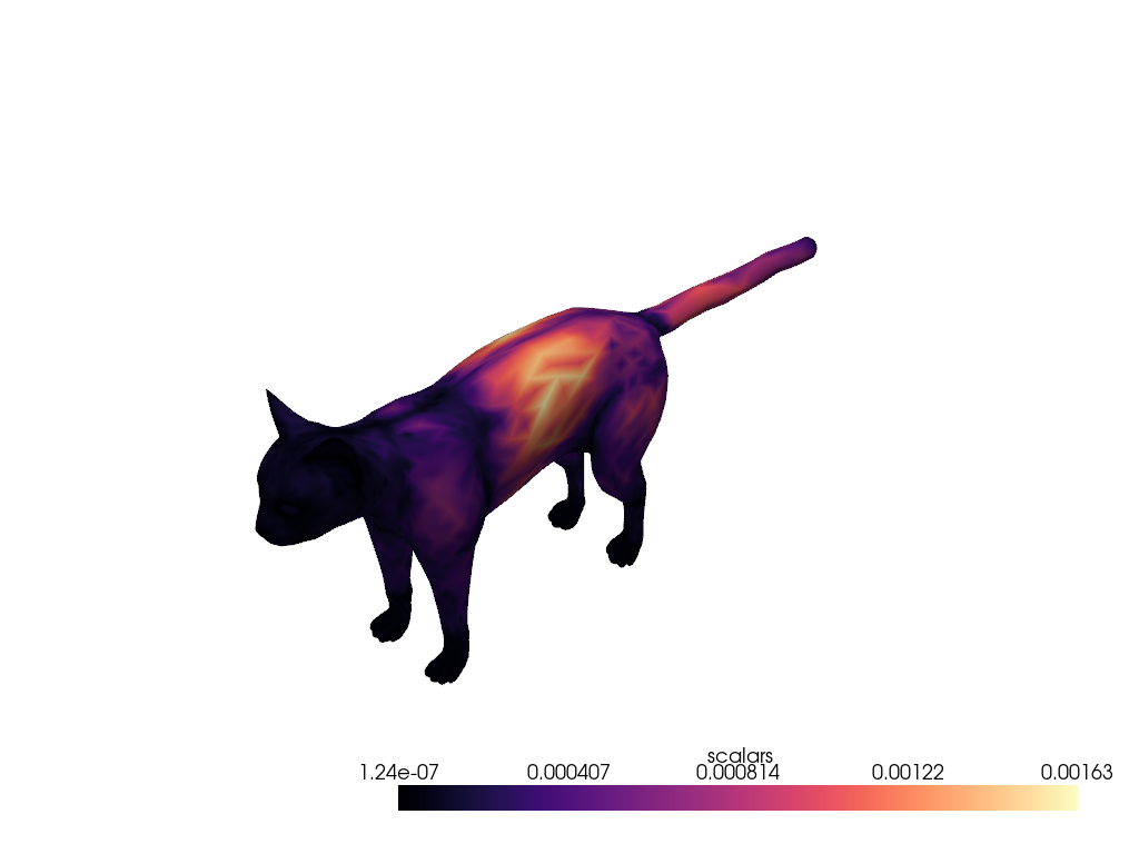
Each face has an area, which is split evenly among the vertices to define vertex areas. Vertex areas define the mass matrix that define inner product and integration of functions on the surface.

print(f"face_areas  : {mesh.face_areas.shape}, sum = {mesh.face_areas.sum():.6f}")
print(f"vertex_areas: {mesh.vertex_areas.shape}, sum = {mesh.vertex_areas.sum():.6f}")

face_areas  : (14410,), sum = 1.000000
vertex_areas: (7207,), sum = 1.000000

Coloring the surface by vertex_areas shows where the triangulation is dense (dark) and where it is coarse (bright).

plot_mesh(mesh, scalars=mesh.vertex_areas, cmap="magma", show_colorbar=True)

Static Scene

Interactive Scene

Normals

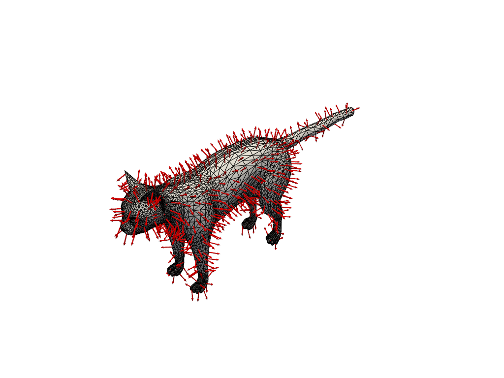
face_normals holds one unit vector per triangle. Passing an array to vfield draws it as arrows, where per-face field is placed at the face barycenters and per-vertex field at the vertices. vfield_tolerance subsamples the arrows to avoid clutter, and vfield_rescale rescales them to a visible length.

plot_mesh(
    mesh,
    vfield=mesh.face_normals,
    vfield_rescale=0.05,
    vfield_tolerance=0.02,
    vfield_color="red",
    wireframe=True,
    line_width=0.5,
)

Static Scene

Interactive Scene

Vertex normals are averages of the adjacent faces, and the averaging weights are a choice. set_vertex_normal_weighting() switches between weighting each face by its area (the default) and weighting them all equally.

The two differ at vertices surrounded by triangles of very different sizes.

normals_area = mesh.vertex_normals.copy()

mesh.set_vertex_normal_weighting("uniform")
normals_uniform = mesh.vertex_normals.copy()

mesh.set_vertex_normal_weighting("area")

cosines = (normals_area * normals_uniform).sum(axis=1).clip(-1, 1)
angles = np.degrees(np.arccos(cosines))

print("angle between the two weightings (degrees):")
print(f"  median {np.median(angles):.2f}, max {angles.max():.2f}")

angle between the two weightings (degrees):
  median 1.09, max 57.75

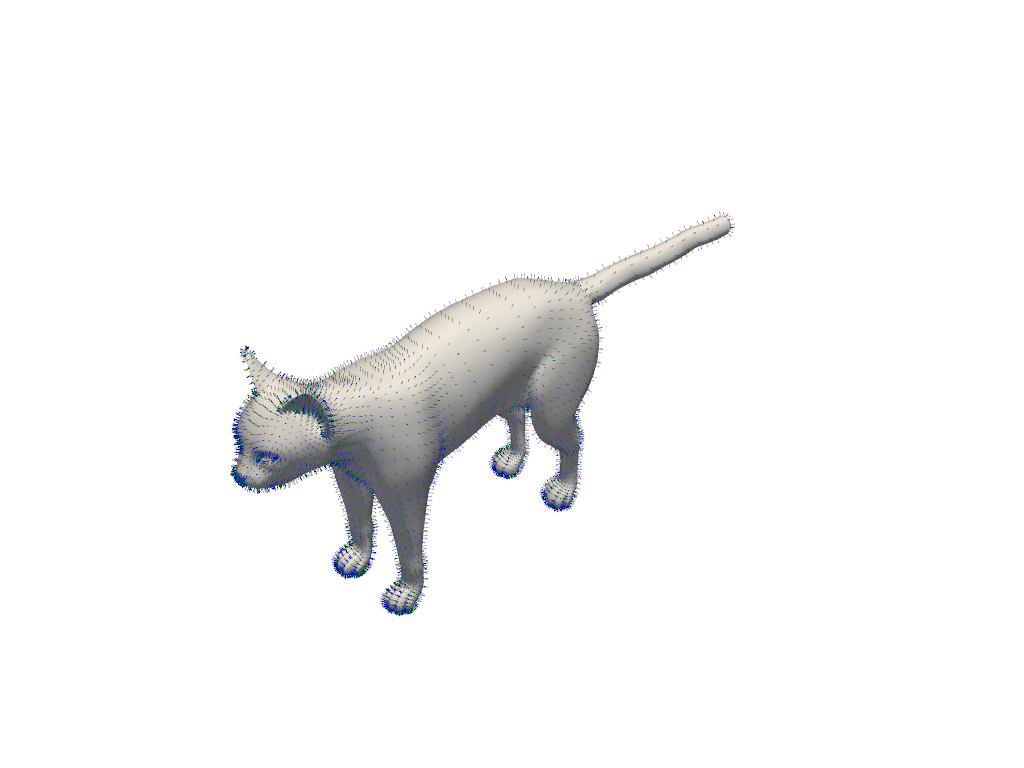
Drawing both fields in one scene makes the agreement visible. To compose plots, plotting function accepts a pl to draw into, and returns one back with return_plot=True.

pl = plot_mesh(
    mesh,
    vfield=normals_area,
    vfield_rescale=0.01,
    vfield_color="blue",
    return_plot=True,
)
plot_arrows(
    mesh.vertices,
    normals_uniform,
    rescale=0.01,
    color="green",
    pl=pl,
)
pl.show()

Static Scene

Interactive Scene

Geodesic distances

geodesic_from() measures distances along the surface from one vertex (or several).

Four methods are available through method=: "heat" (the default, a robust solver from potpourri3d), "heat_pure", "dijkstra" and "fast_marching". The linear systems are prefactorized and reused, so repeated calls on the same mesh are cheap.

points draws spheres on top of the surface.

source = 200
distances = mesh.geodesic_from(source, method="heat")

print(f"distances: {distances.shape}, max = {distances.max():.3f}")

plot_mesh(
    mesh,
    scalars=distances,
    cmap="plasma",
    points=source,
    points_color="red",
    point_size=20,
    show_colorbar=True,
)

Static Scene

Interactive Scene

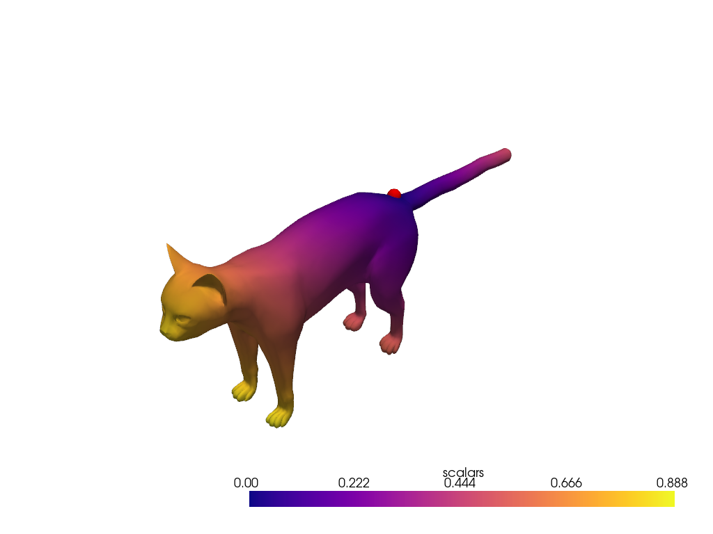
distances: (7207,), max = 0.888

Note

geodesic_matrix() computes all pairwise distances, which is a dense (n, n) array. You can hand it to farthest_point_sampling() to avoid recomputing distances.

Farthest point sampling

farthest_point_sampling() picks a subset of vertices that spreads out over the shape: each new sample is the vertex furthest away from all the previous ones.

Distances are recomputed on the fly unless a full distance matrix is passed as distances. The first sample is drawn at random, so pass distances together with random_init=False when you need the same subset twice.

The function supports both Euclidean and geodesic distances.

samples = mesh.farthest_point_sampling(200, geodesic=True)

print(f"sampled {samples.size} vertices out of {mesh.n_vertices}")

plot_mesh(mesh, color="#b0bec5", points=samples, points_color="crimson", point_size=8)

Static Scene

Interactive Scene

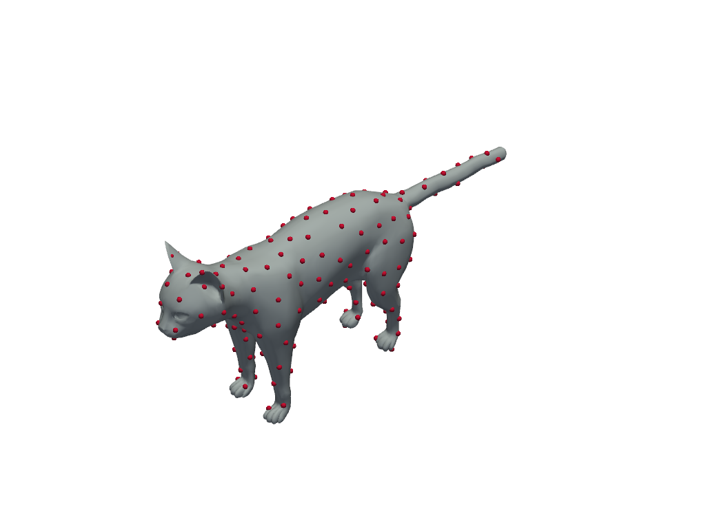
sampled 200 vertices out of 7207

Point clouds

A TriMesh built without faces is a point cloud.

cloud = TriMesh(mesh.vertices)

print(cloud)
print(f"is_point_cloud: {cloud.is_point_cloud}, n_faces: {cloud.n_faces}, area: {cloud.area}")

plot_mesh(cloud, scalars=mesh.vertices[:, 1], cmap="viridis", point_size=4)

Static Scene

Interactive Scene

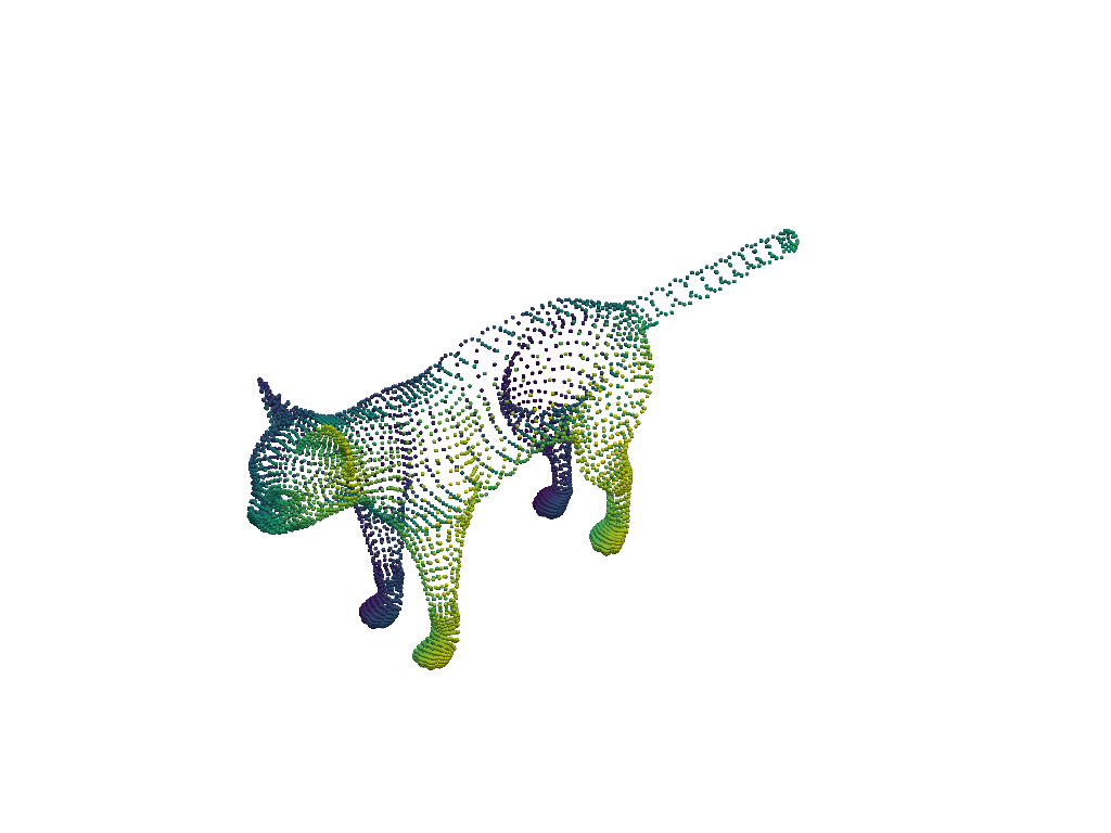
<TriMesh: 7207 vertices (point cloud)>
is_point_cloud: True, n_faces: 0, area: None

Anything that needs the connectivity, such as edges, normals, face areas or geodesic distances, raises a ValueError.

try:
    cloud.face_normals
except ValueError as err:
    print(f"ValueError: {err}")

ValueError: Cannot compute face normals: this mesh has no faces.

The Laplace-Beltrami operator, on the other hand, is still available: pyFM falls back to the robust (tufted) construction, built from the points alone. That operator, and the spectral basis it generates, are the subject of The Laplacian and its spectrum.

Note

The other potpourri3d point cloud operators will be wired in so they work seamlessly on TriMesh point clouds.